
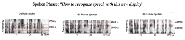
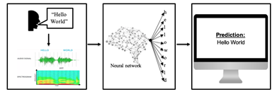
Machine learning is a reasonable approach to recognize and convert speech from spoken words into text because of the different ways a word can sound (Figure 1). As a result, creating a program by hand to try and identify each of the different ways a word could sound is impractical. Instead, a machine learning approach where the model identifies general features to identify spoken words is more feasible. With this in mind, the goal and motivation of this project is to design and train a neural network model that can perform the task of identifying spoken words and convert them into a readable text format (Figure 2).
Data Processing
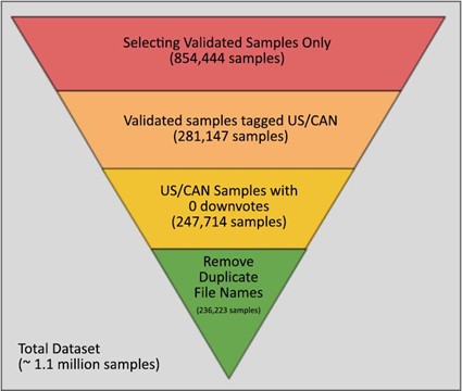
The team collected, cleaned, and completed pre-processing all our sample data. Out of a dataset of over 1.1 million samples from Mozilla Common Voice, we have selected 236,223 samples. Moreover, we have included around 16,000 additional audio samples from Shtooka.
To isolate the data, we applied filters in Excel to the index supplied with the dataset and created a new CSV file listing the filenames of all the selected samples. We extracted the entire dataset and wrote a Python script to move the files to a new directory according to the CSV.
In addition to isolating the sample files, we also cleaned the labels that were provided in the index. Again, Excel was used to remove special characters and punctuation out of the data labels of all the samples. This needed to be done as punctuation marks are not spoken out loud and are outside the scope of our project.
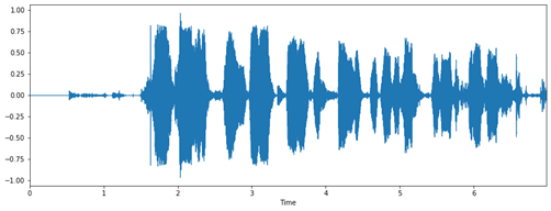
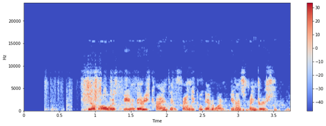
In order to recognize speech, we initially converted our audio files to a general spectrogram, which was to be passed to the RNN as an image classification problem. We made a Jupyter Notebook. We used the Librosa library to perform a Fast Fourier Transform on the audio samples to generate the spectrograms.
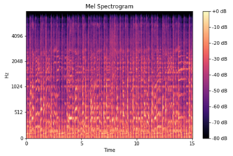
However, we discovered that our primary model was not able to learn much from our original spectrograms, so we decided to try to convert our audio files into Mel Spectrograms. A Mel Spectrogram converts the frequencies into a mel scale, which is a unit of pitch such that equal distances in pitch sounds equally distant to the listener. This is useful because human hearing perceives some frequencies louder than others and allows us to mimic the human hearing.
Architecture & Results
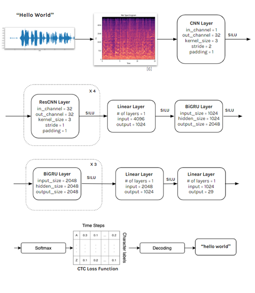
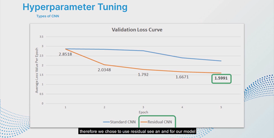
Our model consists of three main neural networks: a convolutional neural network (CNN + ResCNN), a bidirectional gated recurrent unit network (BiGRU), and a fully connected artificial neural network (ANN). Single channel audio clips are first converted into Mel Spectrograms. These are fed through a CNN layer that converts them from a single channel to 32 channels. These are then fed through 4 residual CNN layers, a linear layer, 4 bidirectional GRU layers, 2 linear layers for classification, and then through a softmax function. The output from the softmax function goes through the CTC loss function to calculate the loss and through a decoder which outputs the text version of the speech. SILU activation function is used throughout the model.
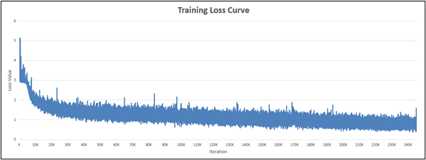
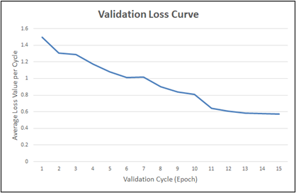
To understand how our model performed quantitatively, we gathered and analyzed the loss values obtained from the CTC loss function during training and validation. Shown in Figure 8, the training loss curve shows a consistent downward trend during a period of over 240 000 iterations (15 epochs). Similarly, Figure 9 shows a validation loss curve that has a consistent downward trend. At the 14th epoch, we observed that the validation loss curve began to flatten out, signalling us that the model was approaching the stopping point and to stop training at the 15th epoch.
Some examples of the model predictions are shown above in Table 1 below. These particular cases were selected as they provide a good overview of the model performance at different epochs. In the initial epochs, the model recognizes words phonetically and attempts to spell them out, which results in predictions with a lot of gibberish. As the training progresses and the number of epochs increase, the model is able to recognize and distinguish between words, and spell them out correctly. Examples of these words include “mineral”, “deposits”, and “backward.” Although the final prediction still contains some misspelled words, the meaning of the statement is not lost as opposed to the initial epochs. Therefore, our model is suitable for some degree of speech recognition.
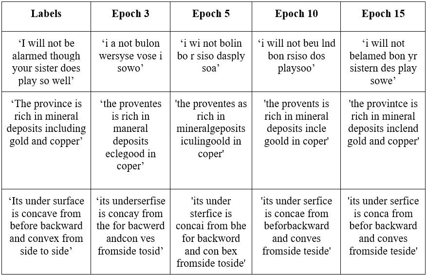
Because our model predicts one character at a time, we only needed to worry about labeling the lower-case English characters and “space”. However, the downside to this is that our model is prone to spelling mistakes (as shown in the qualitative results such as “befor” → before and “concae” → concave). To solve this, we implemented a basic spell checker that is used only during evaluation time. All credits go to Peter and associated authors of the Spelling Corrector code. The spell checker was not used on the predictions in Table 1.
Generating Captions
Using the recorded audio of our presentation, we generated one long transcript using our model. This audio sample was 8 minutes in length, we were able to generate satisfactory results. In our actual presentation, we chose to use another recording where each member recorded their own parts of the presentation while paying very close attention to carefully enunciating every word. This resulted in much better predictions as shown in Figure 10.
Challenges
The difficulty of our project increased due to the following challenges:
Due to our lack of knowledge in the field of speech recognition, we had difficulty developing a model architecture. The initial design consisted only of RNNs, which performed poorly. Progress in the architecture development was eventually made after conducting further research on existing models for speech recognition. Using Assembly AI’s architecture as a basis for our model, we were able to generate a base model and expand on it to overcome this challenge.
It took the model an average of 8 days to complete training. Due to the long training time required and project time constraints, the number of parameters considered for hyperparameter tuning was limited. With more time for experimenting, our model architecture could be fine tuned even further to improve our model predictions.
Ethical Considerations
Potential ethical concerns arise from the way we shaped our dataset. We initially scoped our dataset out of the 1.1 million samples to encompass only samples tagged with a North American (Canada/US) accent, therefore our model may not be very well suited for accents from other countries. Furthermore, since the dataset was collected online, there could be more younger volunteers, therefore resulting in a potential bias towards younger demographics. As such, the limitations to our dataset could result in a bias in the model resulting in poor performance for underrepresented demographics.